8  Appendix 1: Random Walk analysis in R

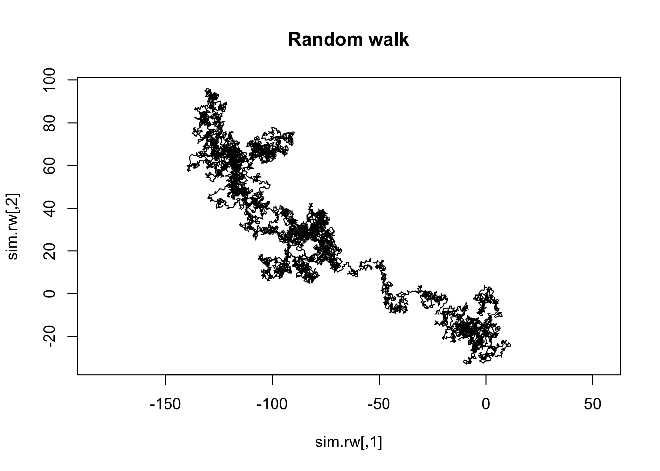
A Random Walk analysis, is a statistical modeling technique used to simulate and analyze sequences of random data points over time.

In a Random Walk, the next data point in the sequence is determined by the current data point plus a random value drawn from a random distribution. The random distribution can be Gaussian (normal), uniform, or any other suitable distribution depending on the application.

8.1 Data import

library(SiMRiv)
rand.walker <- species(state.RW())
sim.rw <- simulate(rand.walker, 10000)
plot(sim.rw, type = "l", asp = 1, main = "Random walk")

8.2 Correlated Random Walk

Define a species with a single-state movement type characterized by a correlated random walk with concentration = 0.98

# simulate one individual of this species
# 10000 simulation steps
c.rand.walker <- species(state.CRW(0.98))
sim.crw <- simulate(c.rand.walker, 10000)
plot(sim.crw, type = "l", asp = 1, main = "Correlated Random walk")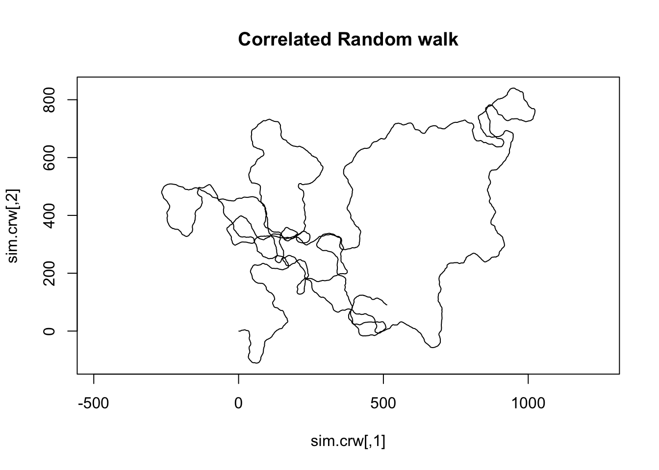

8.3 Application: examples with dummy data

# Load libraries 
  library(SiMRiv)
  library(sf)
  library(terra)
  library(raster)
# Load the "real" data
  wts <- read.csv("data/ex_points.csv")
# Spatial format
  sf_wts <- wts %>% 
    sf::st_as_sf(coords = c(1,2), crs = "+proj=longlat +ellps=WGS84 +datum=WGS84 +no_defs")
  rs_wts <- vect(sf_wts)
# Define the Correlated Random Walk
  c.rand.walker <- species(state.CRW(0.98))
# Create resistance layer
  PUs100 <- st_read("data/PUs_MZ_100km2.shp") # here using the PUs with the different polygons

Reading layer `PUs_MZ_100km2' from data source 
  `/Users/ibrito/Desktop/OceanFrontsChange_Workshop2023/data/PUs_MZ_100km2.shp' 
  using driver `ESRI Shapefile'
Simple feature collection with 65046 features and 1 field
Geometry type: POLYGON
Dimension:     XY
Bounding box:  xmin: 2671147 ymin: -3738837 xmax: 5653079 ymax: -748493.2
Projected CRS: +proj=robin +lon_0=0 +x_0=0 +y_0=0 +datum=WGS84 +units=m +no_defs

  rs_PUs100 <- vect(PUs100) # from sf to terra/raster format
  rs2 <- rast(rs_PUs100, nrow = 3600, ncol = 1800) # create an empty raster
  final <- rasterize(rs_PUs100, rs2, field = "FID") # we need a raster to create the resistance layer
# Binary: # 1 high resistance = no move; # 0 low resistance = move
  final[] <- ifelse(is.na(final[]), 1, 0)
  final2 <- terra::project(final, crs("+proj=longlat +ellps=WGS84 +datum=WGS84 +no_defs")) # the raster needs to be projected...
  final2 <- raster(final2) # the R package SiMRiv not compatible with terra, so we use raster instead
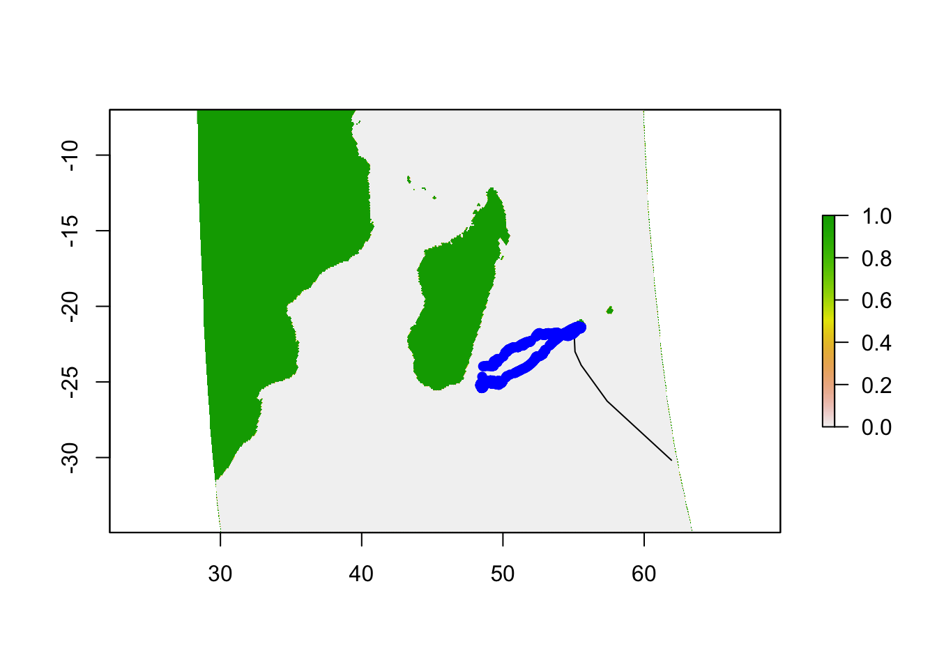
# run the simulation including the resistance layer
  sim.crw <- simulate(c.rand.walker, 
                      time = length(unique(wts$dates)), 
                      coords = as.matrix(wts[1, 1:2]), 
                      resist = final2) # add resist with the land to avoid going into land pixels

# Check and plot the output
  plot(final2)
  lines(sim.crw)
  plot(rs_wts, add = TRUE, col = "blue")