source("zscripts/z_inputFls.R")
source("zscripts/z_helpFX.R") # and the Help function just in case :-)7 Megafauna and Ocean Fronts
7.1 Data import
Source the required dataset.
Or you can actually do the step-by-step.
###################################
####### Whale Shark (mmf dataset)
###################################

# Read the files
  ws01 <- readRDS("data/mm_mmf/MMF_WhaleSharkTracks_Madagascar.rds")
  ws02 <- readRDS("data/mm_mmf/MMF_WhaleSharkTracks_Mozambique.rds")
# Merge
  wsF <- rbind(ws01, ws02) %>%
    dplyr::mutate(group = "Whale Shark")
# Monthly split
  wsF01 <- wsF %>%
    dplyr::filter(dates %in% wsF$dates[stringr::str_detect(string = wsF$dates, pattern = "2016-10.*")])
  wsF02 <- wsF %>%
    dplyr::filter(dates %in% wsF$dates[stringr::str_detect(string = wsF$dates, pattern = "2016-11.*")])
  wsF03 <- wsF %>%
    dplyr::filter(dates %in% wsF$dates[stringr::str_detect(string = wsF$dates, pattern = "2016-12.*")])

  wsF04 <- wsF %>%
    dplyr::filter(dates %in% wsF$dates[stringr::str_detect(string = wsF$dates, pattern = "2011-07.*")])
  wsF05 <- wsF %>%
    dplyr::filter(dates %in% wsF$dates[stringr::str_detect(string = wsF$dates, pattern = "2011-08.*")])
  wsF06 <- wsF %>%
    dplyr::filter(dates %in% wsF$dates[stringr::str_detect(string = wsF$dates, pattern = "2011-09.*")])
  wsF07 <- wsF %>%
    dplyr::filter(dates %in% wsF$dates[stringr::str_detect(string = wsF$dates, pattern = "2011-10.*")])
  wsF08 <- wsF %>%
    dplyr::filter(dates %in% wsF$dates[stringr::str_detect(string = wsF$dates, pattern = "2011-11.*")])
  wsF09 <- wsF %>%
    dplyr::filter(dates %in% wsF$dates[stringr::str_detect(string = wsF$dates, pattern = "2011-12.*")])
7.2 Plotting and testing
# Getting the "help" scripts from source
  source("zscripts/z_inputFls.R")
terra 1.7.39Linking to GEOS 3.11.0, GDAL 3.5.3, PROJ 9.1.0; sf_use_s2() is TRUE
Attaching package: 'dplyr'The following objects are masked from 'package:terra':
intersect, unionThe following objects are masked from 'package:stats':
filter, lagThe following objects are masked from 'package:base':
intersect, setdiff, setequal, union
Attaching package: 'tidyr'The following object is masked from 'package:terra':
extract source("zscripts/z_helpFX.R") # and the Help function just in case :-)
Attaching package: 'patchwork'The following object is masked from 'package:terra':
areaThe legacy packages maptools, rgdal, and rgeos, underpinning the sp package,
which was just loaded, will retire in October 2023.
Please refer to R-spatial evolution reports for details, especially
https://r-spatial.org/r/2023/05/15/evolution4.html.
It may be desirable to make the sf package available;
package maintainers should consider adding sf to Suggests:.
The sp package is now running under evolution status 2
(status 2 uses the sf package in place of rgdal)Support for Spatial objects (`sp`) will be deprecated in {rnaturalearth} and will be removed in a future release of the package. Please use `sf` objects with {rnaturalearth}. For example: `ne_download(returnclass = 'sf')`
Attaching package: 'rnaturalearthdata'The following object is masked from 'package:rnaturalearth':
countries110
Attaching package: 'gganimate'The following object is masked from 'package:terra':
animate
Attaching package: 'transformr'The following object is masked from 'package:sf':
st_normalize
Attaching package: 'data.table'The following objects are masked from 'package:dplyr':
between, first, lastThe following object is masked from 'package:terra':
shiftudunits database from /Library/Frameworks/R.framework/Versions/4.2-arm64/Resources/library/units/share/udunits/udunits2.xmlLinking to liblwgeom 3.0.0beta1 r16016, GEOS 3.11.0, PROJ 9.1.0Loading required package: foreachLoading required package: gifskiLoading required package: ggnewscaleLoading required package: palsWarning: attribute variables are assumed to be spatially constant throughout
all geometries# Pick a random object from above
mmF_test <- wsF01 %>%
st_transform(crs = robin) # always remember to get a common projection!
# Plot
p_test <- ggplot() +
geom_sf(data = mmF_test, colour = "blue", size = 0.3) +
geom_sf(data = world_sfRob, size = 0.05, fill = "grey20")
print(p_test)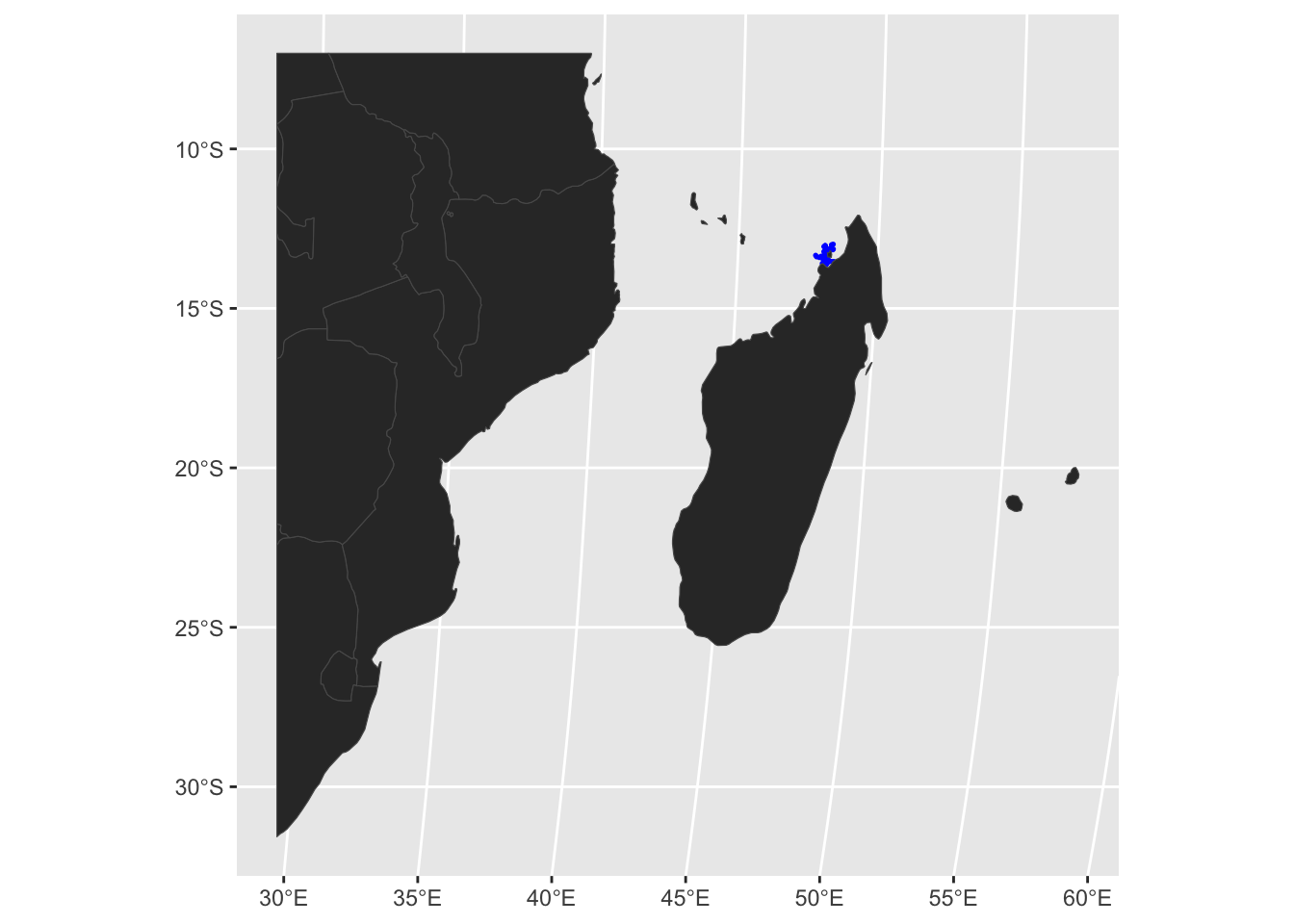
7.3 Near distance to Fronts
source("zscripts/z_inputFls.R")
source("zscripts/z_helpFX.R")

# loading libraries
  library(sf)
  library(terra)
  library(stringr)
  library(dplyr)
  library(data.table)
  library(ggplot2)
  library(patchwork)

# defining the arguments
  pus = "data/PUs_MZ_100km2.shp"
  fsle_sf = "data/fsle_pus_100km2/FSLE_SWIO_2011-12.rds"
  fdata = wsF09
  cutoff = 0.75
  output = "data/"

# Read the front dataset
  PUs <- st_read(pus)
  sf1 <- readRDS(fsle_sf)
  nms <- names(sf1) %>%
    stringr::str_extract(pattern = ".*(?=\\.)")
  colnames(sf1) <- nms

# Matching the appropriate Front data set with the megafauna component
# (from fronts data [sf1] pick the same DATES of megafauna data [fdata])
  df01 <- sf1 %>%
    dplyr::select(as.character(unique(fdata$dates)))

# A loop to match data with front and extract which is the closest value
  Fdates <- unique(fdata$dates)
  FF <- vector("list", length = length(Fdates))
  for(i in seq_along(Fdates)) {
  # Filter the megafauna data for each date
    mmF <- fdata %>%
      dplyr::filter(dates == Fdates[i]) %>%
      st_transform(crs = robin)
  # Filter Front data for each date of the megafauna data
    OFCdates <- df01 %>%
      dplyr::select(as.character(Fdates[i]))
    OFCdates <- cbind(PUs, OFCdates) %>%
      st_transform(crs = robin)
  # Estimate the distance to all
    dist02 <- st_distance(mmF, OFCdates, by_element = FALSE) %>%
      t() %>%
      as_tibble()
    colnames(dist02) <- as.character(mmF$ptt)
  # Get the upper front quantile
    qfront <- OFCdates %>%
      as_tibble() %>%
      dplyr::select(2) %>%
      # as.vector() %>%
      quantile(probs = cutoff, na.rm = TRUE) %>%
      as.vector()
  # First 5 FIRST closest distances to a nearest Front
    dist03 <- apply(X = dist02, MARGIN = 2, FUN = function(x) {
      dist <- x
      final <- cbind(PUs[,1], OFCdates[,2], dist) %>%
        as_tibble() %>%
        dplyr::select(-geometry, -geometry.1) %>%
        dplyr::filter(.[[2]] > qfront) %>%
        dplyr::arrange(.[[3]]) %>%
        dplyr::slice(1:5)
      })
    FF[[i]] <- do.call(cbind, dist03)
  }

# Tidy up the final list
  names(FF) <- Fdates
  FF <- FF[order(names(FF))]

# File name for the output
  ngrd <- unlist(stringr::str_split(basename(pus), "_"))[3] %>%
    stringr::str_remove_all(pattern = ".shp")
  ndate <- unlist(stringr::str_split(basename(fsle_sf), "_"))[3] %>%
    stringr::str_remove_all(pattern = ".rds")
  th <- paste("cutoff", cutoff, sep = "-")
  ffname <- paste("whale-shark_neardist", ngrd, ndate, th, sep = "_")
  saveRDS(FF, paste0(output, ffname, ".rds"))
7.4 Clean (yes, even more!)
dt <- readRDS("data/whale-shark_neardist_100km2_2011-12_cutoff-0.75.rds")
exm <- lapply(dt, function(x) {
  sngl <- x
  df1 <- split.default(sngl, rep(1:(ncol(sngl)/3), each = 3))
  dist1 <- units::set_units(unlist(lapply(df1, function(x2) x2[1,3])), "m")
  dist2 <- as.vector(dist1)})
Fdates <- paste0(unlist(stringr::str_split(names(exm)[1], pattern = "-"))[1:2], collapse  = "-")
#
dst1 <- Reduce(c, exm) %>%
  units::set_units("m") %>%
  units::set_units("km")
lsout <- dst1 %>%
  as_tibble() %>%
  dplyr::mutate(date = as.factor(Fdates)) %>%
  dplyr::rename(neardist = value) %>%
  dplyr::select(date, neardist)
7.5 Distance Histograms
# Getting the dates
  s1 <- lsout
  Fdates <- as.vector(unique(s1$date))

# Plotting
  ff <- ggplot(data = s1,  aes(x = neardist, fill = date)) +
      geom_histogram(data = subset(s1, date == Fdates),
                     aes(x = neardist, y = (..count..)/sum(..count..)),
                     colour = "1",
                     bins = 30) +
      scale_fill_manual(values = c("#2b8cbe"),
                        name = "",
                        labels = Fdates) +
      scale_y_continuous(breaks = seq(0, 1, 0.2), limits = c(0, 1)) +
      coord_cartesian(xlim = c(0, 30)) +
      theme_bw() +
      theme(plot.title = element_text(face = "plain", size = 20, hjust = 0.5),
            plot.tag = element_text(colour = "black", face = "bold", size = 23),
            axis.title.y = element_blank(),
            axis.title.x = element_text(size = rel(1.5), angle = 0),
            axis.text.x = element_text(size = rel(2), angle = 0),
            axis.text.y = element_text(size = rel(2), angle = 0),
            legend.title = element_text(colour = "black", face = "bold", size = 15),
            legend.text = element_text(colour = "black", face = "bold", size = 13),
            legend.key.height = unit(1.5, "cm"),
            legend.key.width = unit(1.5, "cm"),
            legend.position = "none") +
      labs(x = "Distance to high FSLE",
           y = "Density") +
      # geom_richtext(inherit.aes = FALSE,
      #               data = tibble(x = 27, y = 0.8, label = paste("n", "=", nrow(s1), sep = " ")),
      #               aes(x = x, y = y, label = "label"),
      #               size = 6,
      #               fill = NA) +
      ggtitle(Fdates)